Unsteady exact solutionPlanned

Taylor-Green vortex

A decaying array of counter-rotating vortices, and one of the few unsteady flows whose velocity and pressure are both known in closed form for all time.

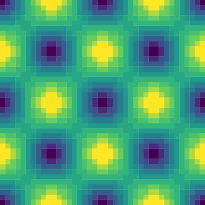
Unsteady2DExact solutionPeriodic

The problem

The Taylor-Green vortex starts from a regular checkerboard of counter-rotating vortices in a doubly periodic box. Nothing drives it, so viscosity simply bleeds energy out of the pattern: every vortex keeps its shape and position exactly, and only its strength decays. The two-dimensional case is one of a very small number of unsteady flows for which the full incompressible Navier–Stokes equations admit a closed-form solution in both velocity and pressure, valid at every instant rather than only in a limit.

That is what makes it worth publishing. The other cases in this group pin down accuracy in space at a steady state, or accuracy in time on a one-dimensional profile. Here the exact answer is available everywhere and at every moment, so space and time error can be measured against the same formula, and a scheme that is second order in one but not the other has nowhere to hide.

It is also the standard place where a real solver and a learned surrogate part company. The decay is exponential and its rate is fixed by viscosity alone, so an answer can be checked against a number nobody has to take on trust.

Exact solution (doubly periodic, kinematic viscosity ν)

u(x,y,t) = -\cos x \, \sin y \; e^{-2\nu t}

v(x,y,t) = \phantom{-}\sin x \, \cos y \; e^{-2\nu t}

p(x,y,t) = -\tfrac{1}{4}\left(\cos 2x + \cos 2y\right) e^{-4\nu t}

What we will measure

The study will run the periodic box on a sequence of uniformly refined meshes, holding the timestep small enough that the time error stays well below the spatial error, and compare the computed velocity against the formula above at a fixed output time. The error is the discrete L2 norm of the difference over every cell, so no single probe point can flatter the result.

A second-order scheme must cut that error by a factor of four for every halving of the cell size, which is a slope of two on log axes. The velocity amplitude decays as the exponential of minus twice the viscosity times time, and the pressure field twice as fast again, so the same run also checks that the solver reproduces the decay rate and not merely the shape of the vortices.

Published results are measured, not predicted. This page carries the problem, the exact solution and the measurement plan; the orders below stay marked pending until the refinement sweep has been run and committed.

Expected result

Nothing below is a measurement yet. The orders and comparisons are what this case is built to test, and each one stays marked pending until the runs are made and committed. Every number published elsewhere in this library traces to a run; these will too.

Spatial order (velocity)Target

Accuracy in space, against the closed-form velocity

expected 2.00→pending

Spatial order (pressure)

Accuracy in space, against the closed-form pressure

expected 2.00→pending

Decay rate

Whether energy leaves the flow at the rate viscosity sets

expected exp(−2νt)→pending

Level	Cells per side	Mesh size h	L2 velocity error
1	32	π/16	pending
2	64	π/32	pending
3	128	π/64	pending
4	256	π/128	pending

The planned refinement sweep, not a result. Each level halves the cell size, so a second-order scheme should divide the error by four down the column.

← All validation cases