Standard Physics

Verification & validation

Proof the numbers are real.

A solver earns trust by measuring its own error. Verification checks that the equations are solved correctly; validation checks that they are the right equations. We do both, we measure the error directly against answers that are known exactly, and we publish it.

Computed temperature field and buoyancy-driven circulation — Boussinesq convection: a field computed by the solver, not a learned prediction.

\begin{aligned} e(h) &= \lVert u_h - u \rVert = C\,h^{\,p} + o(h^{\,p}) \\[8pt] p &= \frac{\log\!\big(e(h_1)/e(h_2)\big)}{\log\!\big(h_1/h_2\big)} \end{aligned}

Discretization error e against the exact solution u, on meshes of size h. The observed order p is the slope on log axes.

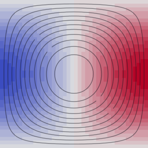
How accuracy is measured

The error must shrink at the rate theory predicts.

The error is measured against the exact answer on finer and finer meshes. It must fall as a fixed power of the cell size, the order of accuracy p: a second-order method has p = 2. We report the observed p for every case.

Order of accuracy

Measured directly against an exact answer.

Four cases with a closed-form answer, each converging at the predicted order. Open any for the method, the equations, and the plot.

Solution field for Kovasznay flow

2D spatial accuracyPass

Kovasznay flowA steady laminar wake behind a two-dimensional grid, one of the few flows with a closed-form solution to the full Navier–Stokes equations.

Spatial order (velocity), expected2.00

Solution field for Ethier–Steinman flow

3D spatial accuracyPass

Ethier–Steinman flowA fully three-dimensional, time-dependent Beltrami flow with an exact Navier–Stokes solution, used to measure spatial accuracy in 3D.

Spatial order (velocity), expected2.00

Solution field for Boussinesq convection

Coupled heat + flow accuracyPass

Boussinesq convectionA buoyancy-driven flow constructed by the Method of Manufactured Solutions to measure accuracy when temperature and momentum are two-way coupled.

Temperature order, expected2.00

Solution field for Stokes’ second problem

Time accuracyPass

Stokes’ second problemA viscous layer driven by an oscillating wall, a classical unsteady benchmark for the accuracy of the time integration.

Temporal order, expected2.00

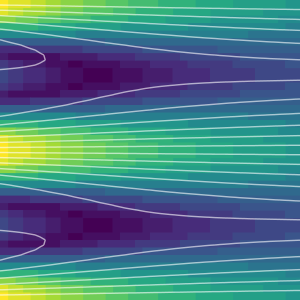
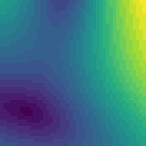
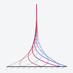
Case studies

Run on real applications.

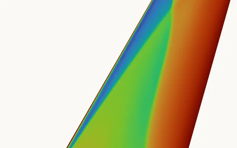
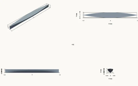
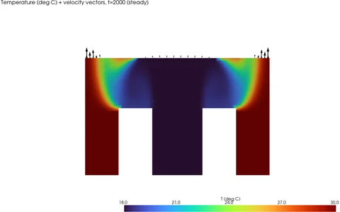
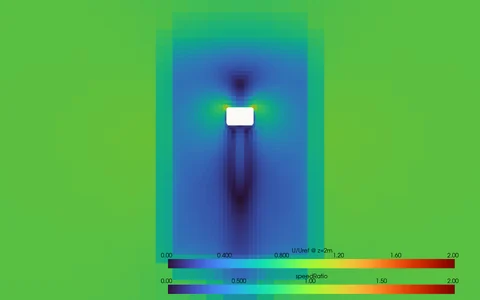
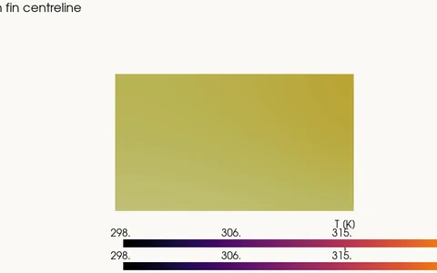
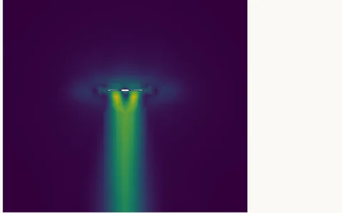
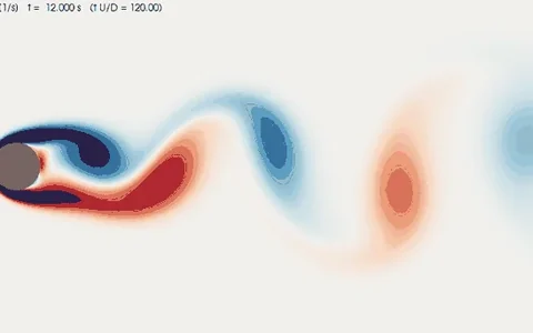
A few of the studies run on Reynolds, across aero, marine, thermal, and the built environment.

ONERA M6 wing

Transonic aeroONERA M6 wing

SUBOFF hull

Marine dragSUBOFF hull

Wigley hull

Free surfaceWigley hull

Data-centre aisle

ThermalData-centre aisle

Pedestrian wind

Built environmentPedestrian wind

Finned heat sink

ElectronicsFinned heat sink

Propeller thrust

PropulsionPropeller thrust

Vortex shedding

UnsteadyVortex shedding

How we check

The method behind the numbers.

Manufactured solutionsKnown-answer testsError measured against an exact answer.

Grid convergenceMesh independenceDistance from the mesh-independent value.

Tested on every changeHundreds of casesRe-run on every change to the solver.

Open and reproducibleStandard formatsCAD/BIM in, VTK out. Reproducible.

Validation on your own application.

We can run the same workflow on your geometry, materials, and operating conditions.

Talk to us Try Reynolds